Chapter 14: Learning from each other

Time elapsed: 20y6m

The failed invasion turned out to be a stroke of luck, as the invaders have taught you a lot about the rest of the world. They come from a huge country that stretches from Europe to Asia, a region that retained more technology and memories of the past than North America did.

‎

They remember more because the area around the Mediterranean Ocean has more people in a smaller area, with dry places nearby that preserve the past better. They don’t know exactly what happened, except that there was once a golden age of technology but then humanity “became arrogant and paid the price”.

‎

Some of them find it funny that Toria is so advanced but still primitive in some areas.

‎

One of them thinks that the news of the defeat will shake up their continent for a while. Europe will soon hear the news, and may start sending teams to Toria to see what they can learn from the people who so quickly destroyed the invading force.

‎

Many who chose to remain are curious about SurrealDB and would like to join your team, and you are happy to show them. They gasp as you turn on the computer and bring up Surrealist in a window and start showing them a few things. It’s a real pleasure to see once again how people react to seeing modern technology for the very first time.

A closer look at Surrealist

This chapter is mostly devoted to looking at Surrealist in more depth, but also gets into some other interesting subjects like table views, grouping, versioned queries, and vector embeddings.

While it’s more than likely that you’ve been using Surrealist for your queries throughout this book, there are quite a few features that aren’t obvious at first glance. In addition, a few of them are only available on the desktop version. The desktop-only features are (unsurprisingly) thanks to the fact that you have access to a computer and its file system when running on a desktop.

For example, only the desktop version of Surrealist has the Start serving and Open console buttons on the top right. Clicking on Start serving will start a SurrealDB database in the same way that the surreal start command does, while Open console shows you the output that you would otherwise see on the command line.

The Surrealist desktop version also has other options besides memory to save your database. This can be accessed inside the Database Serving section of the Settings menu.

File association is another nice feature of the desktop version, because clicking on a .surql or .surrealql file will automatically open it up inside Surrealist on the desktop.

With that advertisement for the desktop version out of the way, let’s start taking a look at each of Surrealist’s views to see what functionality we might have missed and will find helpful to know.

Explorer view

The main purpose of the Explorer view is to allow you to explore the tables and records in your database without needing to put queries of your own together. This point-and-click functionality makes it the ideal first view to choose with for people who are not as tech savvy as you are, but still need to work with data.

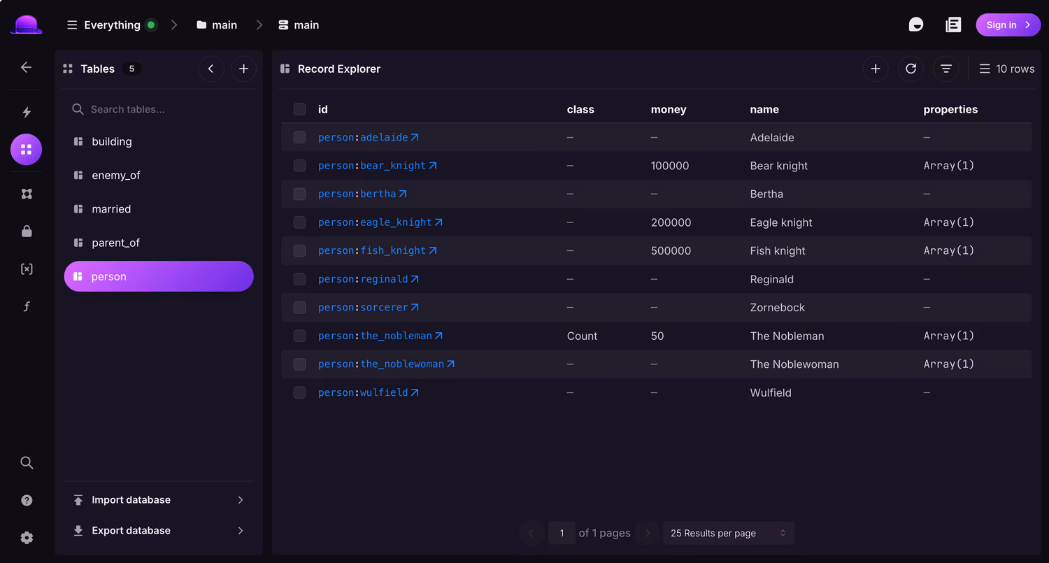
Back in chapter 8, we finished up a multi-chapter project involving most of the characters from the old German story The Enchanted Knights. The project was focused on learning to use the RELATE statement and getting used to graph queries using the -> operator, as well as the beginnings of learning how to define schema. Let’s pull up the dataset from that chapter to see what it looks like inside Surrealist’s Explorer view.

Once the queries inside the dataset are run, you should be able to click on the person table on the left to see the data for all of the person records.

Besides pointing and clicking to see the data for your records, you can also directly modify them. Let’s give that a try with the record for person:adelaide , which should show the following data.

{
  id: person:adelaide,
  name: 'Adelaide'
}

However, Adelaide was the daughter who married the Eagle Knight, so she should be the owner of castle:eagle_castle too! We can add the third line below to make her an owner.

{
    id: person:adelaide,
    name: 'Adelaide',
// +    properties: [building:eagle_castle]
}

Then just click save changes! Just make sure that your changes conform to the schema. If you type something that does not conform to the schema like properties: { building: "Eagle Castle" } and click Save changes, nothing will happen.

Using the Explorer view to visualize relations

The Explorer view is particularly nice when first learning to query on graph tables.

One of the challenges from chapter 8 was to put together a query that shows all of the grandchildren for every person record. Here it is in a similar form, except that we are following the path all the way to their name field.

SELECT 
  ->parent_of->person
  ->parent_of->person.name
FROM person;

We are quite familiar with these queries by now, but the Explorer view lets us try it one step at a time to see what SurrealDB sees at each point. Let’s give this a try. We know that there is only one grandperson in our records, so we’ll start by clicking on person:grandmother .

The table below shows what SurrealDB sees during this query as we continue to follow the path one step at a time. Try following this one step at a time inside the Explorer view.

Note that at the person:reginald part of the query, we went straight to Reginald’s name property. However, we could have easily continued the relation query, because he has two parent_of relations, as well as an enemy_of relation. If we had followed the enemy_of relation, then we would have gotten all of the enemies of the grandchildren of the grandmother.

Here’s another example of a query that we can follow to see how SurrealDB goes through our queries one step at a time.

SELECT
    name,
    properties.name AS property_names,
    ->parent_of->person.name AS name_of_children
FROM person;

We’ll follow the query in the Explorer view by doing this:

• Select any person . Let’s choose person:the_noblewoman .
• SurrealDB now needs to find the value of the name field. It’s right there: ‘The Noblewoman’.
• The next path is properties . The record building:old_castle shows up here. Hold Ctrl and click your mouse button here to get to it. We can see the next path: name , which has the value ‘Old castle’.
• Click the back arrow to get back to person:the_noblewoman . Now we need to check her parent_of relations.
• We can see four outgoing relations here. SurrealDB has to follow these relations, then move out into the person records, and find their name s.

After all this clicking, we have finally simulated the path that SurrealDB follows every time we use a query like this. Putting all the data together, we have an output that looks like this.

{
    name: 'The Noblewoman',
    name_of_children: [
        'Reginald',
        'Wulfield',
        'Bertha',
        'Adelaide'
    ],
    property_names: [
        'Old castle'
    ]
}

Designer view

We’ve learned that defining a schema is the primary way to make your data work in the way that you expect. There is another benefit to it, however: it allows Surrealist to visually display the schema in the Designer view to make it easy for others to follow along.

And more importantly, the Designer view also shows you at a glance where your schema could use some extra definitions.

We can see this by taking a look at the schema from the Chapter 8 dataset that we have been using. The Designer view shows us that the schema is well defined in some areas, but incomplete in others.

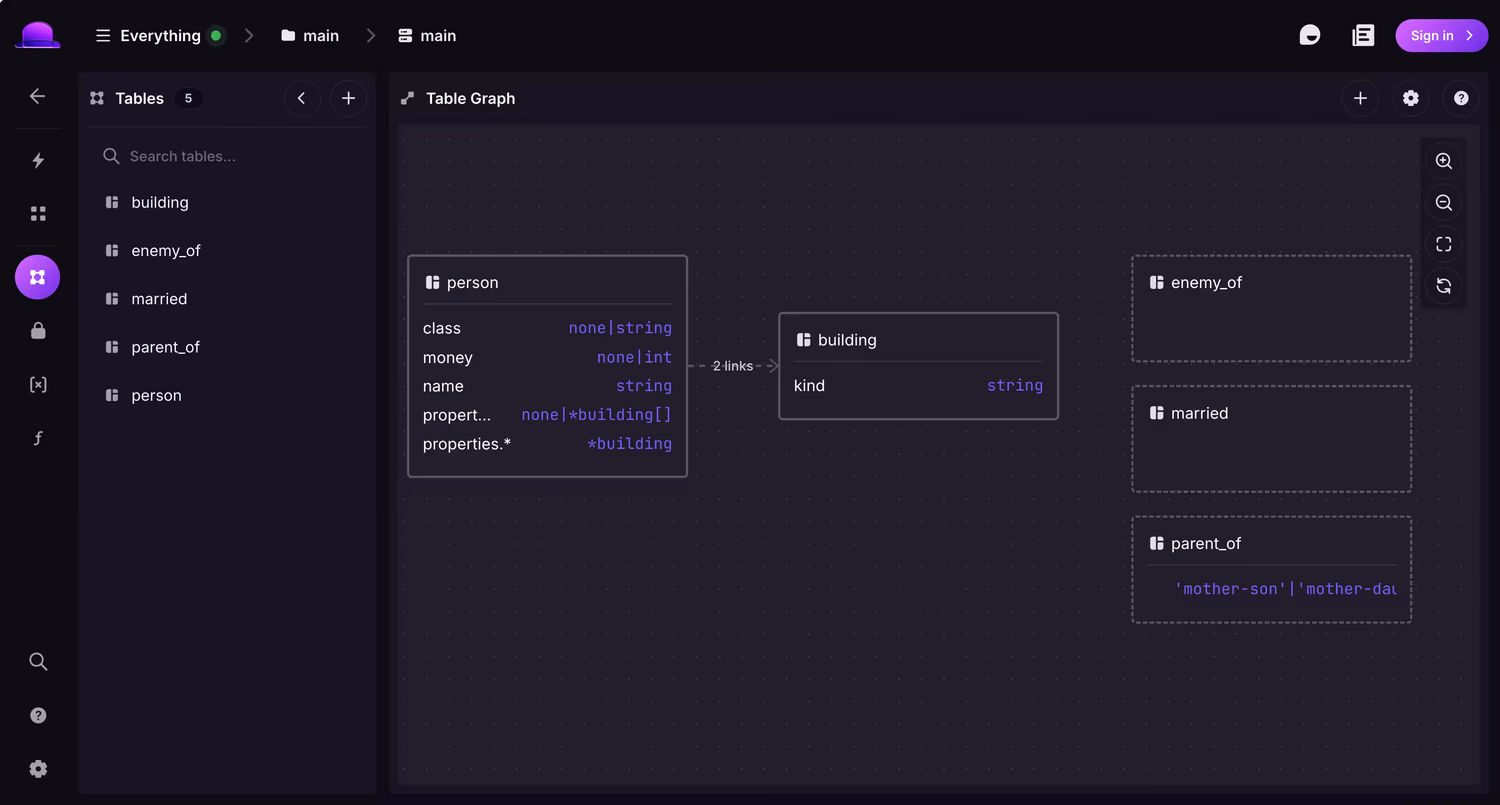
The Designer view shows the defined fields and whether they are optional or not, and moving the mouse arrow over each one will show further details if the field is optional. The properties field also shows that this is a record link to the building table (an array<record<building>> ).

However, SurrealDB doesn’t know what to tell us about the three graph tables: parent_of , married , and enemy_of . We used statements like RELATE person:grandmother->parent_of->person:the_nobleman; to create these tables, but never specifically defined them as relations. They are simply being used as relations.

As we learned in Chapter 9, tables can be defined as relations with the following syntax:

DEFINE TABLE table_name TYPE RELATION IN record_name OUT record_name;

This can also be done through the Designer view too, so let’s practice that.

• Click on parent_of , which should open up the menu to modify its settings.
• Select Enforce schema to make it schemafull.
• The table type is currently Any . Change it to Relation .
• We can now specify what kind of relation is allowed. Change incoming tables to person , and outgoing tables to person .
• Click on Save changes.

All of the other relations are person to person , so we can repeat the same process for married as well as enemy_of .

The resulting schema will now look much better! You can move the objects around with your mouse until they look just right.

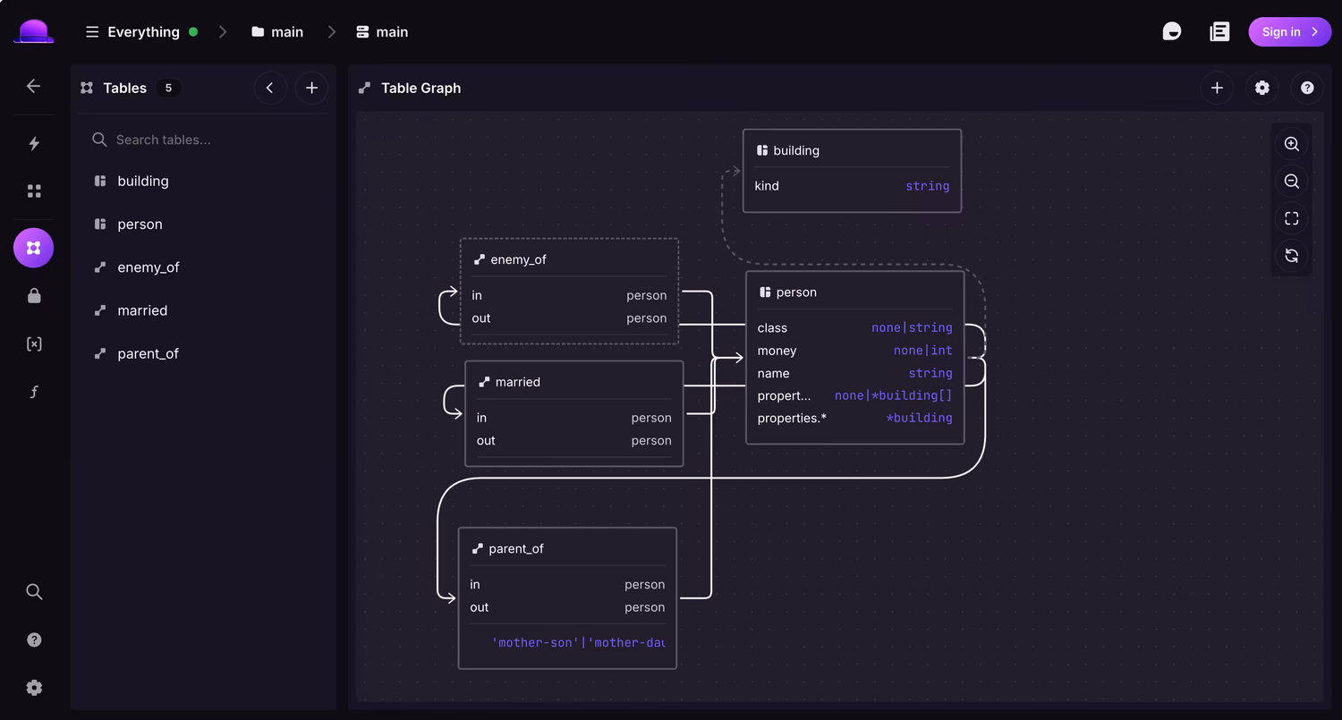
All of these relation tables are from a person to person , so the path leading to each graph table always leads back to a person .

Let’s create a record called city:kago so that we can demonstrate what a relation from one table to a different table looks like. The Designer view should now show a city floating about on its own.

We’ll now create a graph table to connect person and city records. Click on the + button, select Relation, and give the table the name lives_in . The incoming table (the in part of the table) will be a person , and the outgoing table will be a city .

A look at the INFO FOR DB command shows that these tables now have definitions, except that this time we didn’t need to write them manually.

tables: {
    building: 'DEFINE TABLE building TYPE NORMAL SCHEMAFULL PERMISSIONS NONE',
    city: 'DEFINE TABLE city TYPE NORMAL SCHEMALESS PERMISSIONS NONE',
    enemy_of: 'DEFINE TABLE enemy_of TYPE RELATION IN person OUT person SCHEMAFULL PERMISSIONS NONE',
    lives_in: 'DEFINE TABLE lives_in TYPE RELATION IN person OUT city SCHEMAFULL PERMISSIONS NONE',
    married: 'DEFINE TABLE married TYPE RELATION IN person OUT person SCHEMAFULL PERMISSIONS NONE',
    parent_of: 'DEFINE TABLE parent_of TYPE RELATION IN person OUT person SCHEMAFULL PERMISSIONS NONE',
    person: 'DEFINE TABLE person TYPE NORMAL SCHEMAFULL PERMISSIONS NONE'
}

These DEFINE statements bring up another intesting point.

While the Designer view showed us an aspect about the schema that we couldn’t see in the DEFINE statements alone, these staments also show us something that the Designer view alone didn’t tell us: while most tables are of TYPE NORMAL or TYPE RELATION , the city table is of TYPE ANY - which includes relation tables!

In other words, SurrealDB will still let one person “city” another person (whatever that means?).

RELATE person:bertha->city->person:the_nobleman SET name = "Nice city";

The Nobleman gets 'citied' by Bertha
[
  {
    id: city:7zrrq04dm5g548rx7blt,
    in: person:bertha,
    name: 'Nice city',
    out: person:the_nobleman
  }
]

We definitely don’t want that, so let’s click on city and change its table type to Normal.

Having done that, we can’t “city” a person to another person anymore. That’s a relief.

RELATE person:bertha->city->person:the_nobleman SET name = "Nice building", kind = "castle";

Response
'Found record: `city:xwtzzq4krjdvv2nwqje7` which is not a relation, but expected a  NORMAL'

So the best way to make sure that your schema is the way you intended it to be is to use a combination of Surrealist’s Designer view and reading manually through the database’s DEFINE statements.

DROP tables, table views, and grouping

Almost all of the items inside the Table designer inside the Designer view were probably already quite familiar to you, as we have already encountered them in previous chapters. Fields, indexes, even changefeeds and events are nothing new to us at this point.

But what about the “Drop writes to this table” box, what does it do?

The easiest way to find out is with experimentation. Let’s give it a try with a new table. Click on new table, name it weather , keep it schemaless, and then open up the Table designer and click on “Drop writes to this table”. If you check the INFO FOR DB command, you will see the keyword DROP added to the DEFINE TABLE statement for the weather table.

Next, we will create and then select some weather records to see what happens.

DEFINE TABLE weather DROP;
CREATE weather SET temperature = 10.0, location = city:toria;
CREATE weather SET temperature = 15.0, location = city:toria;
SELECT * FROM weather;

The output of the last query seems to show that these weather records are indeed being created, but immediately disappear.

-------- Query --------

[
  {
    id: weather:6o92se7ik3eoe8dq48y6,
    location: city:toria,
    temperature: 10
  }
]

-------- Query --------

[
  {
    id: weather:gwwkii8idbq61gpta7d1,
    location: city:toria,
    temperature: 15
  }
]

-------- Query 3 --------

[]

So that on its own isn’t very useful. However, there is a way to put these weather records to use, with something called a “table view”. A table view is a table that you define using the word AS , followed by a SELECT expression. You can think of a table view as a listener. Once it has been defined, it will continue to respond to new records for the table that it has been defined on.

Let’s give one a try. We’ll call it weather_data . It will use a SELECT on any weather records that we create, and continue to hold on to and add to the result of this expression even if the weather records are immediately dropped.

DEFINE TABLE weather_data AS SELECT * FROM weather;

After this, we can perform a SELECT * FROM weather_data . However, because it was defined after the weather records were dropped, it won’t return anything yet.

No problem! Our weather_data table is already set up and ready to listen for weather table events, so let’s just add a few.

INSERT INTO weather (location, temperature) VALUES
    (city:toria, 10.0), (city:toria, 15.0),
    (city:sukh, 9.5), (city:sukh, 10.1),
    (city:redmont, 16.0);

SELECT * FROM weather_data;

The output shows from SELECT * FROM weather_data shows that this table view is indeed creating new records every time a weather table is created, before the weather data is dropped.

[
  {
    id: weather_data:45thid2180ft0tpnuw17,
    location: city:sukh,
    temperature: 9.5f
  },
  {
    id: weather_data:8usrtp0f0m0v40yndnzr,
    location: city:sukh,
    temperature: 10.1f
  },
  {
    id: weather_data:cs4984kvxy7327dyxqgs,
    location: city:redmont,
    temperature: 16
  },
  {
    id: weather_data:st6nokx48pp226zw9h1w,
    location: city:toria,
    temperature: 15
  },
  {
    id: weather_data:y21yjx69z89n1hu4velq,
    location: city:toria,
    temperature: 10
  }
]

Now let’s make this table view a bit more useful. One way to do so is by using the GROUP BY keyword, which lets us aggregate data to give total count, averages, and so on.

Let’s start with a GROUP BY query that SurrealDB will reject, so that we can see what it expects us to do with this clause. We’ll create some person records, give them an age, and then try to select their id while grouping by age . Note that there are two person records that are 20 years old, and just one that is 45.

CREATE person, person SET age = 20;
CREATE person SET age = 45;
SELECT id FROM person GROUP BY age;

The error here is pretty nice! It tells us that the SELECT part of a GROUP BY expression must contain the fields following GROUP BY , and can also contain an aggregate function.

'There was a problem with the database: Parse error: Missing group idiom `age` in statement selection
 --> [3:32]
  |
3 | SELECT id FROM person GROUP BY age;
  |                                ^^^ 
 --> [3:8]
  |
3 | SELECT id FROM person GROUP BY age;
  |        ^^ Idiom missing here
'

So let’s change the final SELECT query to include only age , and to also group by age .

CREATE person, person SET age = 20;
CREATE person SET age = 45;
SELECT age FROM person GROUP BY age;

The output is now an array with two objects, one for each possible age. Even though there are two person records that have an age of 20, they have been grouped into a single object for the age that they share.

Response
[
  {
    age: 20
  },
  {
    age: 45
  }
]

What makes a GROUP BY clause special is that you can add aggregate functions to the SELECT fields to perform calculations on each group before it is turned into an object. An aggregate function is a function that evaluates an entire array of values, such as count() or math::mean() . Let’s use count() to show that the age: 20 part of the first object actually comes from two records, not one.

CREATE person, person SET age = 20;
CREATE person SET age = 45;
SELECT count(), age FROM person GROUP BY age;

Response
[
  {
    age: 20,
    count: 2
  },
  {
    age: 45,
    count: 1
  }
]

Now that we know how to group, let’s change the name of our weather_data table to weather_averages , and add the average temperatures with the math::mean() function.

DEFINE TABLE weather_averages AS
    SELECT
        location,
        count(),
        math::mean(temperature) AS avg_temp
    FROM weather
    GROUP BY location;

INSERT INTO weather (location, temperature) VALUES
    (city:toria, 10.0), (city:toria, 15.0),
    (city:sukh, 9.5), (city:sukh, 10.1),
    (city:redmont, 16.0);

SELECT * FROM weather_averages;

The output shows us the grouped info, as well as one other interesting point: each record returned also has its own automatically generated id (like weather_averages:[city:toria] ) which represents the grouping we chose.

[
  {
    avg_temp: 16dec,
    count: 1,
    id: weather_averages:[
      city:redmont
    ],
    location: city:redmont
  },
  {
    avg_temp: 9.8dec,
    count: 2,
    id: weather_averages:[
      city:sukh
    ],
    location: city:sukh
  },
  {
    avg_temp: 12.50dec,
    count: 2,
    id: weather_averages:[
      city:toria
    ],
    location: city:toria
  }
]

In addition to GROUP BY , you can choose the GROUP ALL option when you want to get the aggregate values for an entire array of records. Take the following random temperature data for example, which creates 1000 records that each have a random temperature somewhere in between -30 and 40 degrees.

FOR $nothing IN 0..1000 {
    CREATE temp_reading SET
    val = math::round(
      rand() * 40 + -rand() * 30
    );
};

To see the number of items and the average temperature, we can use the math::mean() and count() functions. But if we use GROUP BY for each of these fields, we will get a grouping that shows the number of items that have a temperature of -29 , the number of items with a temperature of -27 , and so on!

FOR $nothing IN 0..1000 {
    CREATE temp_reading SET
    val = math::round(
      rand() * 40 + -rand() * 30
    );
};

SELECT
    math::mean(val) AS mean,
    count() AS num_items
FROM temp_reading GROUP BY mean, num_items;

Response
[
  {
    mean: -29,
    num_items: 2
  },
  {
    mean: -27,
    num_items: 3
  },
  {
    mean: -26,
    num_items: 5
  },
  ...
]

Instead, we can use GROUP ALL so that the aggregate functions work on the full array of records returned instead of splitting into small groups.

FOR $nothing IN 0..1000 {
    CREATE temp_reading SET
    val = math::round(
      rand() * 40 + -rand() * 30
    );
};

SELECT
    math::mean(val) AS mean,
    count() AS num_items
FROM temp_reading GROUP ALL;

With that, the output finally shows the number of items and the average temperature, which will be around 4 or 5 degrees.

[
  {
    mean: 4.762f,
    num_items: 1000
  }
]

Table views offer better performance

Because table views are calculated ahead of time, they offer much better performance when using a large collection of records. We can show this with the example that we’ve just seen. Try running this example below which creates 500 temp_reading records and see what happens when you run it over and over and over again.

You should notice the execution time start to grow, because every time you run the query the database has to begin a table scan of each and every record, and every time there are 500 more of them than before.

LET $now = time::now();
FOR $nothing IN 0..500 {
    CREATE temp_reading SET val = math::round(rand() * 40 + -rand() * 30);
};
-- Assign the SELECT to a variable that we don't read
-- so that we don't have to see the output
LET $nothing = SELECT
    math::mean(val) AS mean,
    count() AS num_items
FROM temp_reading GROUP ALL;
RETURN time::now() - $now;

So let’s replace that with a table view. The table temp_reading will now become a drop table, and the query that we have been using to select and group the data will now be defined as a table called temp_averages .

DEFINE TABLE temp_reading DROP;
DEFINE TABLE temp_averages AS
    SELECT math::mean(val) AS mean,
    count() AS num_items
FROM temp_reading GROUP ALL;

With those definitions in place, let’s keep adding 500 items at a time, but selecting from the pre-computed temp_averages table instead. The increasing delay should be gone now, because all SurrealDB has to do every time we run the queries is create 500 records and update the average a bit.

LET $now = time::now();
FOR $nothing IN 0..500 {
    CREATE temp_reading SET val = math::round(rand() * 40 + -rand() * 30);
};
SELECT * FROM temp_averages;
RETURN time::now() - $now;

With table views and grouping out of the way, let’s take a look at an interesting keyword that you’ll only see with one storage engine for SurrealDB.

SurrealKV and the VERSION keyword

We won’t get into the details of SurrealKV in this book, but there is a single keyword that only SurrealKV can use that you will want to familiarize yourself with: VERSION .

Using the keyword is pretty simple: just add VERSION and a datetime to queries like CREATE and SELECT .

CREATE something VERSION d"2024-09-15";
SELECT * FROM something VERSION d"2024-09-16";

Neither of these queries will work when using SurrealDB in memory or another storage layer, and it won’t work in the runnable Surrealist embed either. Instead, you’ll see the following error.

'The underlying datastore does not support versioned queries'

As we learned back in Chapter 3, we can start a database with a certain storage layer by giving it a path that begins with the name of the layer to use. So if we add surrealkv:somedatabase to the surreal start command, it will recognize that we want to use SurrealKV and create a database with the path somedatabase . To make sure that versioning isn’t enabled for users who don’t need it, it is disabled by default. To run SurrealKV with versioning, add +versioned just before the path, like this:

surreal start --user root --pass root surrealkv+versioned:somedatabase

Once this command has started a new database instance, we can try these queries with VERSION again. First we’ll create a bunch of some something records, each with a different datetime after VERSION .

CREATE something VERSION d"2024-09-16";
CREATE something VERSION d"2024-09-17";
CREATE something VERSION d"2024-09-18";

SELECT * FROM something;

The final SELECT query shows that this VERSION keyword hasn’t done anything to the visibile data, as each record simply has an id and nothing else.

[
  {
    id: something:mbei8oll3jjvcwt6rjy6
  },
  {
    id: something:ou0t498qyi7r0mmy0d5g
  },
  {
    id: something:s49tjrkau10kc2a701ve
  }
]

However, if we add VERSION and a datetime to the final SELECT query, we can see something interesting: instead of returning each record, it returns a snapshot of all these records as of that date.

Let’s go back in time to the morning of September 17th, 2024. It’s 9 o’clock UTC and Londoners are drinking their morning tea. What did our something records look like as of that date? Let’s find out.

SELECT * FROM something VERSION d"2024-09-17T09:00:00Z";

The answer is…just two of them! Even though the database currently holds three.

[
  {
    id: something:ou0t498qyi7r0mmy0d5g
  },
  {
    id: something:s49tjrkau10kc2a701ve
  }
]

Note that with a VERSION that includes future dates, a query will default to returning the current state of all the records. So this query that includes a VERSION of for the 17th of September 2024 will return these three something records, even though later on the same query might show more than that. SurrealDB isn’t (yet??) capable of predicting what records will be there in the future.

SELECT * FROM something VERSION d"2024-09-17T09:00:00Z";

Aeon and the team will certainly be using SurrealKV as their storage layer, since the dates they use in their calendar (it’s currently the year 444 for them) work perfectly well as datetimes!

CREATE financial_transaction CONTENT {
  -- lots of important data here
} VERSION d"0444-04-19";

We are quickly approaching the end of the chapter, but it looks like Aeon has just discovered something else that is very relevant to the AI-crazed world we currently live in. Let’s see what this discovery is.

Vector embeddings

Later that day…

You found something interesting in one of your office computers this afternoon: a whole bunch of files in the format called JSON. JSON itself is no mystery to you, but one of the fields grabbed your attention.

‎

The JSON objects in these files hold thousands and thousands of strings with information, famous quotes, and just about anything you can think of. But the interesting part is a field called embedding . This field takes up most of the screen space and is nothing but one small number after another, like 0.0056326561607420444f. There are hundreds of them for each piece of text.

‎

After enough searching through the documentation, you realize that these numbers represent some sort of “mental location” for the quote. And that SurrealDB has a way to work with them!

‎

This could be useful. Time to see how these numbers work.

Looks like Aeon has discovered vector embeddings! While there are no services in Aeon’s day like OpenAI and Mistral, these already stored embeddings on a computer will work just as well for a limited dataset.

What are vector embeddings?

To start, we will make sure that we understand what vector embeddings are so that we aren’t left behind. Let’s grab some of the Shakespeare quotes from Aeon’s files and see what they look like. The output below shows some text along with an array of floats. In practice, this array of floats will have hundreds or even thousands of values, but we’ll cut it them down to three for readability.

[
	{
		embedding: [
			0.0007022718782536685,
			0.004178352188318968,
			0.009888353757560253
		],
		text: "To be, or not to be: that is the question."
	},
	{
		embedding: [
			-0.027426932007074356,
			0.0008020889363251626,
			-0.02949262224137783
		],
		text: "All the world’s a stage, and all the men and women merely players."
	},
	{
		embedding: [
			-0.05859993398189545,
			-0.011999601498246193,
			-0.06185592710971832
		],
		text: "The course of true love never did run smooth."
	}
]

These numbers represent the “semantic space” for the input, namely the approximate space for the meaning that it holds.

First of all, where do these numbers come from anyway?

They come from language models. Companies like OpenAI and Mistral have services that will take an input from you, returning you a big array of floats to represent its semantic space. The output depends entirely on the model.

The competition between these companies is based on which ones have the best models, the ones that represent semantic space the best. Companies that have developed particularly accurate models will get more people willing to pay them for the service, and that’s how they continue to make money and improve the models as time goes on.

There are a lot of open source models too such as the models available through fastembed or the Transformers library (available here as well in Rust), which can run directly on your machine instead of calling into a service. And there are models for other types of input such as images, sound, and so on.

Vector embedding basics

The following three phrases show how semantic space works. Notice that the first and second sentence are visually close to each other, because they use a lot of the same words: “Surrealist” and “Surrealists”, and the word “visual”. But semantically (in terms of meaning) the last sentence is much closer, because it also discusses a way to use a program to access a database - even if it doesn’t have a single word that matches the words in the first sentence.

• “Surrealist, the visual app for SurrealDB”
• “Surrealists were popular in the aftermath of World War I and strongly impacted the visual arts”
• “A terminal interface to access a database”

As humans we know that sentences one and three have the closest meaning to each other, but let’s prove it through embeddings.

First, copy the content here into Surrealist which holds each of those three sentences along with their embeddings. It also includes the embeddings for the word “SurrealDB” on its own. It will insert four document records that each have the original text as well as an embedding for each.

Using them, we can do a search to see the distance or similarity between them. It’s a little bit like full-text search, except in a more visual way (if you are a computer, that is). These functions are found inside the vector module.

Once you go to that page you’ll notice that there are a ton of choices to make. This is because there are many ways of computing the distance between something.

To understand why there might be more than one way to measure distance, think about the stars in the sky. Looking in the sky, you might see two stars that are close to each other. But in reality, they are very likely not close to each other at all: they only look close to you, who is standing on the planet Earth and looking their way. This apparent distance is the Cosine distance.

If you want to take into account that one star is 5 light-years away and the other is 5000 light years away, even if they look close to each other, then that’s the Euclidean distance.

And there are many other ways to calculate distance, as you can see in this reference guide on vectors.

But don’t worry, because Cosine is the usual way to measure semantic distance or similarity. For the time being, you can just pretend that Cosine is the only way to calculate distance between embeddings. To do so in SurrealDB, we can use the vector::similarity::cosine() function. Its input and output looks like this.

RETURN vector::similarity::cosine([10, 50, 200], [400, 100, 20]);

0.15258215962441316f

Now let’s try to use it with the document records that we inserted. Here is how we will build up the query to use it.

First, grab every document record and call .map() . This is because we want to do a similarity search across all the other document records for each document we have.

(SELECT * FROM document).map(|$doc| {

});

Then we will pass on the original text, and a field called compared_to that will show the results of the vector search. To make the original text show up first, we can rename it alphabetically or even just put an underscore in front because an underscore comes before all other letters of the alphabet.

(SELECT * FROM document).map(|$doc| {
    _text: $doc.text,
    compared_to: // Search query goes in here...
});

Finally, we have the search query. It will show the original text , then call vector::similarity::cosine to compare the embedding field of this document with the other document . We will use the alias similarity to give this field a nicer name, and then ORDER BY similarity DESC to show the closest results first. Finally, we will wrap it all in parentheses and use [1..] to return only the items starting from the first index. That’s because the SELECT statement will also compare the current document against itself, which will always have a similarity of 1 , and we don’t need to see that. We only care about the other documents that have different text.

(SELECT text, vector::similarity::cosine($doc.embedding, embedding) AS similarity FROM document ORDER BY similarity DESC)[1..]

Putting that all together gives us this query.

(SELECT * FROM document).map(|$doc| {
    _text: $doc.text,
    similar: (SELECT text, vector::similarity::cosine($doc.embedding, embedding) AS similarity FROM document ORDER BY similarity DESC)[1..]
});

The output looks pretty good! The items returned match with the way we would probably order them ourselves as humans. One interesting part is the text starting with “Surrealists were popular in the aftermath of…”, because there aren’t really any good matches for it in our four document records. So while it does have a closest match with “Surrealist, the visual app for SurrealDB”, it’s still not that similar with a similarity of 0.55. Conversely, the similarity between the “Surrealist…” and “SurrealDB” strings is very close at 0.86. They aren’t just the closest to each other, but objectively semantically close to each other too.

[
	{
		_text: 'Surrealist, the visual app for SurrealDB',
		similar: [
			{
				similarity: 0.8607534612007887f,
				text: 'SurrealDB'
			},
			{
				similarity: 0.6187632165848997f,
				text: 'A terminal interface to access a database'
			},
			{
				similarity: 0.5525827506089576f,
				text: 'Surrealists were popular in the aftermath of World War I and strongly impacted the visual arts'
			}
		]
	},
	{
		_text: 'Surrealists were popular in the aftermath of World War I and strongly impacted the visual arts',
		similar: [
			{
				similarity: 0.5525827506089576f,
				text: 'Surrealist, the visual app for SurrealDB'
			},
			{
				similarity: 0.5377259574881328f,
				text: 'SurrealDB'
			},
			{
				similarity: 0.346735666829385f,
				text: 'A terminal interface to access a database'
			}
		]
	},
	{
		_text: 'SurrealDB',
		similar: [
			{
				similarity: 0.8607534612007887f,
				text: 'Surrealist, the visual app for SurrealDB'
			},
			{
				similarity: 0.601792455902042f,
				text: 'A terminal interface to access a database'
			},
			{
				similarity: 0.5377259574881328f,
				text: 'Surrealists were popular in the aftermath of World War I and strongly impacted the visual arts'
			}
		]
	},
	{
		_text: 'A terminal interface to access a database',
		similar: [
			{
				similarity: 0.6187632165848997f,
				text: 'Surrealist, the visual app for SurrealDB'
			},
			{
				similarity: 0.601792455902042f,
				text: 'SurrealDB'
			},
			{
				similarity: 0.346735666829385f,
				text: 'Surrealists were popular in the aftermath of World War I and strongly impacted the visual arts'
			}
		]
	}
]

In that case, you might want to just return nothing if no similarity is high enough. Here, you could use another .map() to return the original output if any numbers are above a certain similarity (like 0.6), and NONE for the similar field if nothing is high enough.

LET $results = (SELECT * FROM document).map(|$doc| {
    _text: $doc.text,
    similar: (SELECT text, vector::similarity::cosine($doc.embedding, embedding) AS similarity FROM document ORDER BY similarity DESC)[1..]
});

$results.map(|$r| {
    IF $r.similar.any(|$comp| $comp.similarity > 0.6) { 
      $r 
    } ELSE { 
      { _text: $r._text, similar: NONE }
    };
});

We’ve only scratched the surface of how to work with vector embeddings in SurrealDB, but hopefully this has made the subject familiar enough to get started! If you want a longer look at all the other ways to work with them, see the Vector search reference guide.

In the next chapter, we will learn about configuring the users of your database and keeping it safe.