Chapter 10: The ancient world begins to reappear

Time elapsed: 6y

The most frustrating thing for you is that you are aware of the great inventions of the past, but have no idea how to recreate them. Electricity, the airplane, the internet…all of those are beyond your reach. Yes, you have access to a modern network of computers, but you don’t know the first thing about how to make your own!

‎

But you do have one recent success that you are most proud of. It’s called the Chappe Telegraph, and was invented in a country called France. It doesn’t need any electricity, and is surprisingly straightforward. Here is how it works:

‎

• Build a tower with three connected rods on top that bend to form a large number of shapes. Each shape symbolizes a different word.
• Give each tower two telescopes: one to look forward, and another to look backward.
• Build another tower a few kilometres away that the operators can see through the telescope.

All the tower operators have to do is make the same shape as the tower before it every time they see a change. People at the destination then copy the shapes down and use a code book to turn the symbols back into words.

‎

And just like that, it is now possible to communicate from Toria to Black Bay and even as far as The Naimo in just an hour! Your next job is to set up telegraphs on each of the islands across the bay to reach the city of Redmont.

‎

In the meantime, you and many others have become quite used to the measurements of the past and are finding them quite convenient. They are certainly much more precise than your traditional units like “stride” and “thumb” for length, “stone” and “halfweight” for weight, and “period” for time!

Geo functions

It looks like the people of Aeon’s part of the world will soon be ready to move from medieval maps to something more precise. To make sure we are not left behind when they do, we’ll learn about SurrealDB’s geo functions in this chapter and the next one. These functions are all based on GeoJSON, which defines a number of shapes that can be used to calculate distance, area, and so on. A GeoJSON object is composed of a type for the type of shape it is, and coordinates to indicate the points in space to create it. Here is one example:

{
    "type": "LineString",
    "coordinates": [
        [30.0, 10.0],
        [10.0, 30.0],
        [40.0, 40.0]
    ]
}

SurrealDB’s geo functions have pretty simple signatures. Two of them take two points as an argument:

• geo::distance(), which calculates the distance in metres between two points.
• geo::bearing(), which calculates the direction to travel to reach the next point.

The other two take a geometry (a shape):

• geo::area(), which calculates the surface area of a shape.
• geo::centroid(), which calculates the centre of a shape.

The easiest function to understand and use is geo::distance(), so we will start with that. The most important point to know here is that the order is longitude, latitude (also known as “eastings”, “northings”), not latitude, longitude. This is because the GeoJSON spec has defined its inputs in this order.

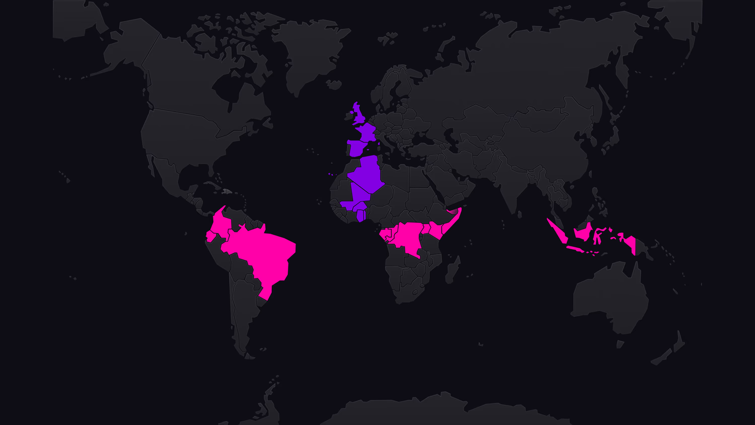
Longitudes to the east of the International Reference Meridian are positive, and longitudes to the west are negative. Latitudes on the north half of the globe are positive, and latitudes to the south are negative. That means that most countries will have numbers that stay either positive or negative, while a few countries that straddle these lines will have numbers that vary from positive to negative.

If you search for the location of London for example, and get this output:

51.5072° N, 0.1276° W

It will become a point containing these two numbers in the opposite order. A tuple of two numbers is recognized by SurrealDB as a geoJSON point. We can prove this by putting these coordinates into the type::is::geometry() function.

-- Returns true
RETURN (-0.1276, 51.5072).is_geometry();

Another way to get a location is by right clicking anywhere in Google Maps or OpenStreetMap, which will let you copy the location at that point. Here is another point inside London:

51.50919990282684, -0.11196686685079893

Turn these around and put them inside a tuple, and you have a point! Let’s also remove some of the digits at the end during this chapter for readability, because we don’t need to be incredibly precise.

RETURN (-0.1119, 51.5091);

You can also construct a Point by following the geoJSON spec, which SurrealDB will return as two numbers.

RETURN [(-0.1119, 51.5091),
{
    "type": "Point",
    "coordinates": [
        -0.1119,
		51.5091
    ]
}];

“surql title=“Response” [ (-0.1119, 51.5091), (-0.1119, 51.5091) ]

Now that we know how to construct a `Point`, let's use this method to see how far the capitals of the Western Roman Empire (Rome) and the Eastern Roman Empire (Constantinople, now Istanbul) were to each other.

Double clicking on these two cities in Google Maps gives us the following points:

41.8924, 12.9271 40.6899, 28.9505

Now we just need to turn them around, put them into tuples, and stick them into the `geo::distance()` function.

```surql runnable=""
RETURN geo::distance(
    (12.9271, 41.8924),
    (28.9505, 40.6899)
);

The output is 1343408.4453224381f, about 1,340 kilometres. You can right click and then select Measure Distance inside Google Maps to see that this is indeed the distance between the two cities.

Next is geo::bearing(), which couldn’t be easier! It also takes two points, so all you need to do is change the word distance in the example above to bearing.

RETURN geo::bearing(
    (12.9271, 41.8924),
    (28.9505, 40.6899)
);

The output this time is 90.3601045887473f, showing that Istanbul is almost directly east of Rome.

Now let’s use LET to create a variable for each point to make our next query to compare the bearing from Rome to Istanbul and from Istanbul to Rome more readable. Interestingly, the bearing from Point A to Point B is not simply the opposite of the bearing from Point B to Point A. This is due to things like the curvature of the Earth and the formula used to perform the calculation that we don’t need to learn in this book.

LET $rome     = (12.9271, 41.8924);
LET $istanbul = (28.9505, 40.6899);

RETURN {
    rome_to_istanbul: geo::bearing($rome, $istanbul),
    istanbul_to_rome: geo::bearing($istanbul, $rome)
};

Response
{
	istanbul_to_rome: -79.02669237408213f,
	rome_to_istanbul: 90.3601045887473f
}

Now let’s get to the other two functions, which take a larger range of inputs than just two points. Instead, they take a geometry. A geometry is some sort of a shape, of which a Point is one. Other types of geometries include LineString and Polygon, and other combinations of these two: MultiPoint, MultiLineString, MultiPolygon, and finally GeometryCollection which holds multiple geometries.

The most common type of geometry used after Point is Polygon, which is what we will use for the next two functions.

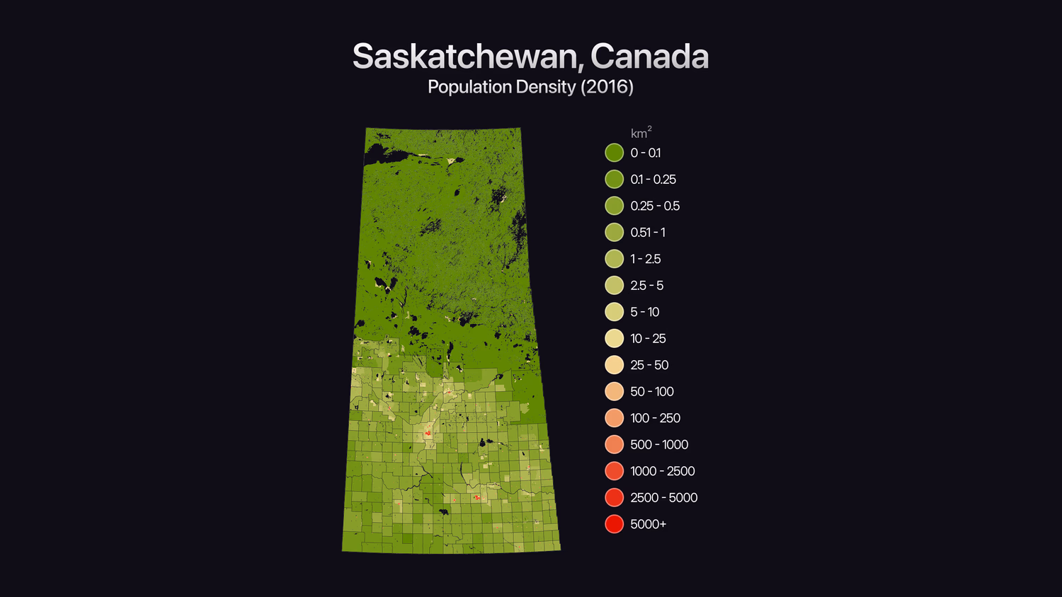
The next function we will look at is geo::area(), which gives the area of a geometry. This is easiest for us to test if we find a nice rectangular piece of territory that will only need a Polygon of four points to approximate. Let’s go with the Canadian province of Saskatchewan, which has a nice boring rectangular shape.

Clicking on its four corners gives us some good approximate numbers. Here they are reversed:

-110.0006, 59.9872
-102.0861, 59.9947
-101.3903, 48.9766
-109.9867, 49.0249

With these points ready to go, all we need to do is put them into the function! Don’t forget to specify the input as a “Polygon”, and then just put the coordinates in. Note the double square brackets inside coordinates as well for an array of arrays, not just one array. This is because the function can also take complex types like MultiPolygon, which requires arrays of arrays.

RETURN geo::area({
	type: "Polygon",
	coordinates: [[
        [-110.0006, 59.9872],
        [-102.0861, 59.9947],
        [-101.3903, 48.9766],
        [-109.9867, 49.0249]
    ]]
});

The output is…651898892358.2931f! This is a pretty close match to Saskatchewan’s official surface area of 651,900 km². Its shape is so rectangular that these four points were enough to almost match perfectly.

And now for the exciting part: the geographic centre of Saskatchewan! Where could it be? Finding it couldn’t be easier, because once again all we have to do is change the function name.

RETURN geo::centroid({
	type: "Polygon",
	coordinates: [[
        [-110.0006, 59.9872],
        [-102.0861, 59.9947],
        [-101.3903, 48.9766],
        [-109.9867, 49.0249]
    ]]
});

The output of this function is a Point.

Response
(-105.86010100139671, 54.42038629153207)

If we go to Google Maps again, we can see that this is indeed the centre! There is even a small detour that allows people passing through to stop for a moment and ponder the wonder of being right in the centre of Saskatchewan.

Geohashes

There are two more functions left to learn, both of which deal with something called a geohash. Geohashes were invented in 2008 in order to turn rectangular spaces of land into short strings of letters and digits.

Let’s start with an example to see how geohashes work. We’ll go with the Parthenon in the centre of Athens, which has survived for 2500 years and is very likely still standing during Aeon’s time as well.

If you right click on the centre of the Parthenon inside Google Maps, you will get a number like this:

37.97153324769507, 23.726653194839038

Now let’s turn the numbers around to put them into a point, which we’ll pass into the geo::hash::encode function.

RETURN geo::hash::encode((23.726653194839038, 37.97153324769507));

This returns the output swbb5bt0pnff, which is 12 digits in length. That’s a geohash.

Now try changing the last digit in the second number of the point from 7 to 8.

RETURN geo::hash::encode((23.726653194839038, 37.97153324769508));

We get swbb5bt0pnff, the same output! With this we can see that a geohash isn’t a cryptographic hash meant to hide input (which we will learn more about in Chapter 15), but just a convenient shorthand.

The longer the length of a geohash, the greater the precision. We can give this a try with the geohash we have and the geo::hash::decode() function, which turns a geohash into a Point. Look what happens as we make it shorter and shorter:

RETURN geo::hash::decode('swbb5bt0pnff');
RETURN geo::hash::decode('swbb5bt0pn');
RETURN geo::hash::decode('swbb5bt0');
RETURN geo::hash::decode('swbb5b');
RETURN geo::hash::decode('swbb');
RETURN geo::hash::decode('sw');
RETURN geo::hash::decode('s');

As the geohash decreases in size, it represents a larger rectangular area of land and is thus less precise.

Response
(23.726653140038252, 37.97153321094811)
(23.726654648780823, 37.971531450748444)
(23.726520538330078, 37.97158241271973)
(23.7249755859375, 37.97149658203125)
(23.73046875, 38.056640625)
(28.125, 36.5625)
(22.5, 22.5)

Here is another way to visualize our geohash that began with a point inside Athens:

• The rectangle ‘s’ represents a huge area from western to eastern Europe and down to the west and east side of central Africa.
• This rectangle ‘s’ is divided into further rectangles. One of them is ‘w’. Together they make ‘sw’, which spans a much smaller area: Greece, Turkey, Cyprus, and so on.
• This rectangle is divided into further rectangles, and so on and so forth.

This handy table will help you decide how many digits you need to store in a geohash for it to be useful.

The Parthenon is about 70 metres across, so a precision of 10 digits or even 9 digits is probably good enough.

Geometries and operators

One really useful part of a geohash is that it allows you to quickly determine if one location is contained in the same zone as another one.

For example, take these geohashes for four cities in Ireland.

RETURN [
	// Dublin
    geo::hash::encode((-6.1971555689385, 53.42134668221924)),
	// Limerick
    geo::hash::encode((-8.590306690257298, 52.70463210234539)),
	// Cork
    geo::hash::encode((-8.501730637251514, 51.92118887515803)),
	// Galway
    geo::hash::encode((-9.06855268816339, 53.33052233370851))
];

Notice how easy it is to compare the items inside the output?

Response
[
	'gc7xfvp3gucc',
	'gc3gud8dxre0',
	'gc1zqecnz745',
	'gc3x3ss2z3vj'
]

A single glance tells you that all of these locations are inside g, then inside c, and only after then do they differ. And because the precision at the second level (where they all match) is 1,252.3km x 624.1km but the precision at the third level (where none of them match) is 156.5km x 156km, you know immediately that these places are fairly close but still a few hours’ drive away from each other.

But be sure to remember that geohashes are only rough estimates, because they refer to rectangular regions. Some locations are located close to each other but across the border, and will seem to be far apart when they actually may be quite close. Take Cambridge and Northampton for example:

RETURN [
	// Cambridge
    geo::hash::encode((0.12828879218748016, 52.22088932116364)),
	// Northampton
    geo::hash::encode((-0.8910089824568541, 52.26533564501211)),
];

The distance from one to the next is a mere 70 km, but one lies inside ‘u’ and the other inside ‘g’, because both of them are close to the border of their own geohash.

Response
[
	'u1214ft2tr74',
	'gcr37dx5tuxx'
]

So when you see a precision of 5,009.4km x 4,992.6km, remember that this includes very short distances as well! The only guarantee we have from these two geohashes is that Cambridge and Northampton are somewhere within about 5000 km of each other, when really they are very close.

Similarly, both Detroit and San Francisco are in the “zone” of the United States, while Windsor and Vancouver are both in the “zone” of Canada. But Detroit is right across the river from Windsor, so being in a different “zone” gives a false impression of distance in this case too.

If you ever have any doubts, be sure to use the geo::distance function to get the real story.

RETURN geo::distance(
    geo::hash::decode('u1214ft2tr74'),
    geo::hash::decode('gcr37dx5tuxx')
);

As it shows, the distance from Cambridge to Northampton is 69575.20061823408f, so about 70 km.

SurrealDB’s CONTAINS and INSIDE operators also work for geometries. Remember the Canadian province of Saskatchewan? Its capital Regina is located at the following geohash.

RETURN geo::hash::encode((-104.6268, 50.4620));

Response
'c8vx54m46ye7'

We can use these operators to check not only whether a point is inside a geometry, but also another geometry.

LET $saskatchewan = {
	type: "Polygon",
	coordinates: [[
        [-110.0006, 59.9872],
        [-102.0861, 59.9947],
        [-101.3903, 48.9766],
        [-109.9867, 49.0249]
    ]]
};
RETURN geo::hash::decode('c8vx54m46ye7') INSIDE $saskatchewan;

LET $regina = {
	type: "Polygon",
	coordinates: [[
		[-104.7713, 50.5136],
		[-104.5402, 50.5113],
		[-104.5649, 50.3977],
		[-104.7622, 50.3978]
	]]
};
RETURN $saskatchewan CONTAINS $regina;

Comparing values and complex record ID behaviour

Now that Toria and Redmont are able to communicate across the bay, they can exchange information such as weather conditions.

Let’s test this by inserting some temperature values for a table called weather and query for records that match the city of Toria along with temperatures between 10 and 20 degrees.

INSERT INTO weather (at, temperature, date) VALUES
    (city:toria,   15, "175-07-01"),
    (city:toria,   18, "175-07-02"),
    (city:toria,   16, "175-07-03"),
    (city:redmont, 16, "175-07-01"),
    (city:redmont, 17, "175-07-02");

SELECT * FROM weather WHERE at = city:toria AND temperature IN 10..20;

No surprise here! This sort of query is very easy for us by now.

[
	{
		at: city:toria,
		date: '175-07-03',
		id: weather:03sul655v8shc9r5zl6r,
		temperature: 16
	},
	{
		at: city:toria,
		date: '175-07-02',
		id: weather:3hc4p0mjoje01c53xslr,
		temperature: 18
	},
	{
		at: city:toria,
		date: '175-07-01',
		id: weather:y5s8r81ohjiiw18xljie,
		temperature: 15
	}
]

But SurrealDB also allows us to do range queries on the id field of a record itself, such as all the records from person:1 to person:10. This works on any sort of record ID, including complex ones.

There are four main options when using range syntax in SurrealDB.

• low..high for up to but not including a value (an exclusive range). person:1..person:10 would return everything up to but not including person:10.
• Changing .. to ..= for up to and including a value (an inclusive range). person:1..=person:10 would return everything up to as well as person:10.
• Changing .. to ..> for from but not including a value (an exclusive range). person:1>..=person:10 would return everything from person:2 to person:10.
• .. (if not followed by anything) for an unbounded range. person:1.. would return everything equal to or greater that person:1, ..=person:10 would return anything up to and including person:10, and so on. And a single .. creates a range that includes everything.

We’ll try this behaviour with three cities: Toria, Redmont, and Black Bay.

CREATE city:toria, city:redmont, city:black_bay;

// From redmont and up to but not including toria
SELECT * FROM city:redmont..toria;
// From redmont and up to and including toria
SELECT * FROM city:redmont..=toria;
// Everything starting from black_bay
SELECT * FROM city:black_bay..;

Response
-------- Query --------
[
	{
		id: city:redmont
	}
]

-------- Query --------

[
	{
		id: city:redmont
	},
	{
		id: city:toria
	}
]

-------- Query --------

[
	{
		id: city:black_bay
	},
	{
		id: city:redmont
	},
	{
		id: city:toria
	}
]

That was fairly straightforward, as those simple IDs were in alphabetic order. Now what about more complex IDs? Let’s give these a try with some weather data.

INSERT INTO weather (id) VALUES
    ({temperature: 19.0, humidity: 55.0}),
    ({temperature: 15.0, humidity: 40.4}),
    ({temperature: 28.7, humidity: 90.5});

And now we can select all the records between certain temperature and humidity, such as temperatures between 0.0 and 20.0 degrees, and humidity between 0.0 and 70.0 degrees.

INSERT INTO weather (id) VALUES
    ({temperature: 19.0, humidity: 55.0}),
    ({temperature: 15.0, humidity: 40.4}),
    ({temperature: 28.7, humidity: 90.5});

SELECT * FROM weather:{
    temperature:0.0,
    humidity: 0.0
}..={
    temperature: 20.0,
    humidity: 70.0
};

[
	{
		id: weather:{
			humidity: 40.4f,
			temperature: 15
		}
	},
	{
		id: weather:{
			humidity: 55f,
			temperature: 19
		}
	}
]

However, this next query returns a result that may be surprising. At first glance, it looks like it will return every weather record that matches a temperature of 0.0 to 20.0 and a humidity up to 70.0…

INSERT INTO weather (id) VALUES
    ({temperature: 19.0, humidity: 55.0}),
    ({temperature: 15.0, humidity: 40.4}),
    ({temperature: 28.7, humidity: 90.5});

SELECT * FROM weather:{
    temperature:0.0
}..={
    temperature: 20.0,
    humidity: 70.0
};

But the output is []!

To understand how this works, we will first need to learn how SurrealDB compares values, arrays, and objects with each other.

The first concept to learn is that everything returned from SurrealDB is a value, and every value can be compared with another. We can show this with the following query that returns true, instead of an error such as “Cannot compare a string to an int”.

RETURN 'Aeon' > 10;

This is because every value internally has an order that goes as follows, from least to greatest:

none
null
bool
number
string
duration
datetime
uuid
array
object
geometry
bytes
record

So any string will be greater than any number, null will always be greater than any none, any duration will be greater than any string, and so on. We can show this with the following query that returns true for every comparison:

RETURN [
    null > none,
    true > null,
    1 > true,
    'a' > 999999999,
    1s > 'a',
    time::now() > 1s,
    rand::uuid() > time::now(),
    [] > rand::uuid(),
    {} > [],
    (89.0, 89.0) > {},
    <bytes>'Aeon' > (89.0, 89.0),
    person:aeon > <bytes>'Aeon'
];

You don’t have to remember each of these types and their order, and indeed, there is probably no situation in which you might want to compare a type like bytes with a string, to choose a random example. But there is one important point to remember here: no value is less than none, which makes it a useful starting point for a range query.

Here is a very quick demonstration of the behaviour, in which we query on a record range that starts with NONE to ensure that every record is returned. This example is meant to be as simple as possible, because we will soon encounter another record range behaviour that we need to understand.

CREATE timestamp:[time::now()];
SLEEP 10ms; -- Make sure that the next time::now() is unique
CREATE timestamp:[time::now()];
CREATE timestamp:[NONE];

SELECT * FROM timestamp:[NONE]..;

Response
[
	{
		id: timestamp:[
			NONE
		]
	},
	{
		id: timestamp:[
			d'2024-06-26T04:45:22.948Z'
		]
	},
	{
		id: timestamp:[
			d'2024-06-26T04:45:22.959Z'
		]
	}
]

The next example is a bit more complex, with a table called conditions that includes both a timestamp and the humidity.

INSERT INTO conditions (id) VALUES
    ({ at: time::now(), humidity: 66.5 }),
    ({ at: time::now(), humidity: 50.0 }),
    ({ at: NONE,        humidity: 34.7 }),
    ({ at: time::now(), humidity: NONE }) RETURN NONE;

SELECT * FROM conditions:{
    at: NONE,
    humidity: 55.0,
}..;

The output returns three records. The only one that does not show up is the one with a lower humidity than 55.0.

Response
[
	{
		id: conditions:{
			at: d'2024-06-26T04:52:56.460Z',
			humidity: NONE
		}
	},
	{
		id: conditions:{
			at: d'2024-06-26T04:52:56.460Z',
			humidity: 50f
		}
	},
	{
		id: conditions:{
			at: d'2024-06-26T04:52:56.460Z',
			humidity: 66.5f
		}
	}
]

However, note what happens when we change the name of the at field to time. Nothing else has changed, but the output is quite different! This time, only a single record is returned.

SELECT * FROM conditions:{
    time: NONE,
    humidity: 55.0,
}..;

Response
[
	{
		id: conditions:{
			humidity: 66.5f,
			time: d'2024-06-26T04:55:39.129Z'
		}
	}
]

We can understand why this happens if we remember that the output of a value is always ordered. Take a look at what happens when we insert one conditions record that has the fields at and humidity, and another that has the fields time and humidity.

INSERT INTO conditions (id) VALUES
    ({ at:   time::now(), humidity: 66.5 }),
    ({ time: time::now(), humidity: 50.0 });

Response
[
	{
		id: conditions:{
			at: d'2024-06-26T04:57:49.742Z',
			humidity: 66.5f
		}
	},
	{
		id: conditions:{
			humidity: 50,
			time: d'2024-06-26T04:57:49.742Z'
		}
	}
]

The output shows up in alphabetical order: at followed by humidity for the first, and humidity followed by time for the second. Internally, SurrealDB stores records in an ordered format which it uses to compare one to another.

So that means that the range query above that included time and humidity was actually interpreted as humidity and then time!

SELECT * FROM conditions:{
    time: NONE,
    humidity: 55.0,
}..;

This concept is easiest to remember if you think of a range query as SurrealDB constantly checking to see if one value is greater or less than another. Take the following two objects for example, which also have a time and a humidity field:

LET $cond1 = { time: NONE,        humidity: 55.0 };
LET $cond2 = { time: time::now(), humidity: 50.0 };
RETURN [$cond1, $cond2, $cond1 > $cond2];

The output shows us how SurrealDB sees it: an object with a humidity and then a time field. The humidity of the first is 55.0, which is greater than the second at 50.0, so even though the first one has a NONE for time, SurrealDB has already concluded that the first is greater than the second because its humidity field has a larger value.

[
	{
		humidity: 55f,
		time: NONE
	},
	{
		humidity: 50f,
		time: d'2024-06-26T05:18:32.541Z'
	},
	true
]

In addition, you also need to ensure that one object is compared with another object of a similar structure. Take the following query for example:

INSERT INTO conditions (id) VALUES
    ({ at: time::now(), humidity: 66.5 }),
    ({ at: time::now(), humidity: 50.0 }),
    ({ at: NONE,        humidity: 34.7 }),
    ({ at: time::now(), humidity: NONE }) RETURN NONE;

SELECT * FROM conditions:{
    humidity: 55.0,
}..;

The output is…nothing! This is because SurrealDB begins by comparing the at field of the conditions records to the humidity field of the object we pass in to the range operation, but at can’t be compared to humidity.

To resolve this, we can pass in an at: NONE into the query so that the structure is the same. SurrealDB will return three conditions records: all except the one which has NONE for the at field and 34.7 for the humidity field, making it lesser than the object we passed into the range operation.

INSERT INTO conditions (id) VALUES
    ({ at: time::now(), humidity: 66.5 }),
    ({ at: time::now(), humidity: 50.0 }),
    ({ at: NONE,        humidity: 34.7 }),
    ({ at: time::now(), humidity: NONE }) RETURN NONE;

SELECT * FROM conditions:{
    at: NONE,
    humidity: 55.0,
}..;

Response
[
	{
		id: conditions:{
			at: d'2024-06-26T05:27:49.105Z',
			humidity: NONE
		}
	},
	{
		id: conditions:{
			at: d'2024-06-26T05:27:49.105Z',
			humidity: 50
		}
	},
	{
		id: conditions:{
			at: d'2024-06-26T05:27:49.105Z',
			humidity: 66.5f
		}
	}
]

Record range queries on complex record IDs using arrays work in a similar fashion, except that SurrealDB moves from one index to the next instead of in alphabetical order. As you can see, they are quite a bit easier to read and reason about because you don’t have to think about the names of fields.

INSERT INTO conditions (id) VALUES
    ([time::now(), 66.5]),
    ([time::now(), 50.0]),
    ([NONE,        34.7]),
    ([time::now(), NONE]);

SELECT * FROM conditions:[NONE, 55.0]..;

Aeon is going to be busy over the next few years continuing to grow this new network of telegraph towers. In the next chapter, we’ll see how the world has changed as a result.

[-80.54, 41.97],
[-75.00, 41.70],
[-75.41, 39.78],
[-80.50, 39.72]

RETURN geo::centroid({
  type: "Polygon",
  coordinates: [[
	[-80.54, 41.97],
	[-75.00, 41.70],
	[-75.41, 39.78],
	[-80.50, 39.72]
  ]]
});

LET $centre = (-77.9292, 40.8094);
LET $philly = (-75.1636, 39.9528);

RETURN geo::distance($centre, $philly);

LET $centre = (-77.9292, 40.8094);
LET $philly = (-75.1636, 39.9528);

RETURN geo::bearing($centre, $philly);
RETURN geo::bearing($philly, $centre);